PART IV – Introductory methods for scoring analysis
At face value, California edged out in front of Chile, overall. In a basic competition, scores would be totalled up or, even further, averages would be calculated to declare a winner – quite simple. But do these comparisons go far enough? Can we say with certainty that if we were to repeat these flights with other groups over and over again (and you know how we’d love to!) that California would remain on top?
Statistical sip #1 – Averaging and standard error
I never thought that statistics could be this much fun to work with until using them in a wine context. The number crunching becomes even more enjoyable with a refreshing glass in hand! Taking a look at the breakdown, the individual scores are below along with an average. Accompanying the average is another measure known as standard error of the mean (SEM) which is one of many ways to describe the spread, or how much each of the scores vary from one another. If the SEM was zero, the scores would be completely identical. If the scores varied greatly, then the SEM would also be much greater. I labelled each wine as either from California (CAL) or Chile (CHL).
Table 1: Flight 1 – Individual scores, average and standard error (out of 8 tasters)
| A | B | C | D | E | F | |
|---|---|---|---|---|---|---|
| La Follette | Veramonte | Santa Carolina | Rodney Strong | Gloria Ferrer | Errazuriz | |
| CAL | CHL | CHL | CAL | CAL | CHL | |
| Chard | Chard | Cabsauv | Cabsauv | Pnoir | Pnoir | |
| 16 | 11 | 11 | 17 | 16 | 15 | |
| 15 | 10 | 15 | 15 | 17 | 14 | |
| 19 | 12 | 12 | 16 | 16 | 15 | |
| 17 | 11 | 12 | 16 | 18 | 14 | |
| 18 | 9 | 13 | 5 | 17 | 15 | |
| 15 | 10 | 18 | 10 | 13 | 14 | |
| 18 | 15 | 14 | 19 | 19 | 18 | |
| 17.1 | 11.3 | 13.4 | 14.4 | 16.5 | 14.9 | AVERAGE |
| 0.6 | 0.6 | 0.8 | 1.6 | 0.6 | 0.5 | SEM |
Table 2: Flight 2 – Individual scores, average and standard error (out of 12 tasters)
| A | B | C | D | E | F | G | H | |
|---|---|---|---|---|---|---|---|---|
| Errazuriz Mx | Ch. St. Jean | Cakebread | Maycas Limarí | Chilcas | Dierberg | Dom. Napa | V. San Esteban | |
| CHL | CAL | CAL | CHL | CHL | CAL | CAL | CHL | |
| Svblanc | Svblanc | Chard | Chard | Pnoir | Pnoir | Cabsauv | Cabsauv | |
| 11 | 13 | 13 | 19 | 13 | 18 | 19 | 16 | |
| 12 | 12 | 13 | 18 | 14 | 19 | 18 | 17 | |
| 14 | 16 | 12 | 16 | 15 | 18 | 19 | 15 | |
| 11 | 11 | 12 | 16 | 14 | 12 | 18 | 14 | |
| 3 | 12 | 10 | 16 | 16 | 17 | 16 | 17 | |
| 9 | 6 | 14 | 14 | 11 | 17 | 17 | 18 | |
| 14 | 15 | 13 | 17 | 14 | 17 | 13 | 18 | |
| 15 | 16 | 12 | 16 | 17 | 17 | 14 | 13 | |
| 13 | 12 | 15 | 18 | 16 | 15 | 19 | 17 | |
| 12 | 11 | 16 | 17 | 15 | 15 | 18 | 15 | |
| 14 | 10 | 12 | 16 | 17 | 15 | 15 | 14 | |
| 15 | 17 | 12 | 18 | 16 | 18 | 19 | 17 | |
| 11.9 | 12.6 | 12.8 | 16.8 | 14.8 | 16.5 | 17.1 | 15.9 | AVERAGE |
| 1.0 | 0.9 | 0.5 | 0.4 | 0.5 | 0.6 | 0.6 | 0.5 | SEM |
With a closer look at the numbers one can tell that in some matchups Chile actually beat California. In other pairings the scores were almost tied with a difference of less than one point. So now, going beyond calculating an average for the raw scores, let’s use some rudimentary statistics to further analyze the tasting.
Statistical sip #2 – Corrected score, removing the outliers
You’ve often seen this in figure skating, or at least suspect it, where one or more judges score far from their peers. In wine tasting, it is possible that one or more judges are just having a great day and score a wine as though it’s made from angel tears. On the other hand, there might be another that caught a really bad cold and can’t taste anything at all, scoring the wines far below the panel average. By removing the top and bottom outliers we arrive at a more representative average. Also, notice how the SEM becomes smaller because we’ve essentially removed some of the spread. Statisticians have many ways to select which values to tag as outliers for removal, some of these methods involve mathematical complexities that should only be discussed over a fine bottle of port (and a full bottle, if one wishes to keep their companion’s attention) so we’ll just keep it simple – no method is the best method.
Table 3: Flight 1 – Corrected average and standard error (out of 6 tasters)
| A | B | C | D | E | F | |
|---|---|---|---|---|---|---|
| La Follette | Veramonte | Santa Carolina | Rodney Strong | Gloria Ferrer | Errazuriz | |
| CAL | CHL | CHL | CAL | CAL | CHL | |
| Chard | Chard | Cabsauv | Cabsauv | Pnoir | Pnoir | |
| 17.2 | 11.0 | 13.0 | 16.7 | 16.7 | 14.5 | AVG SCORE |
| 0.6 | 0.4 | 0.5 | 0.6 | 0.3 | 0.2 | SEM |
Table 4: Flight 2 – Corrected average and standard error (out of 10 tasters)
| A | B | C | D | E | F | G | H | |
|---|---|---|---|---|---|---|---|---|
| Errazuriz Mx | Ch. St. Jean | Cakebread | Maycas Limarí | Chilcas | Dierberg | Dom. Napa | V. San Esteban | |
| CHL | CAL | CAL | CHL | CHL | CAL | CAL | CHL | |
| Svblanc | Svblanc | Chard | Chard | Pnoir | Pnoir | Cabsauv | Cabsauv | |
| 12.5 | 12.8 | 12.8 | 16.8 | 15.0 | 16.7 | 17.3 | 16.0 | AVG SCORE |
| 0.6 | 0.7 | 0.3 | 0.3 | 0.4 | 0.4 | 0.6 | 0.4 | SEM |
Statistical sip #3 – Visualizing the spread
One can visualize the judges’ scores by simply charting the average score into a point and using bars to depict the size of that standard error we discussed earlier. Here’s one set of many possible examples:
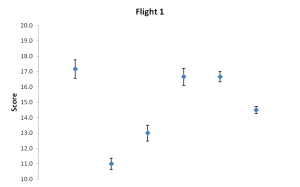
Scores in chart format with dots representing the average score and the bars depicting the spread as a standard error. Wines A through F (left to right).
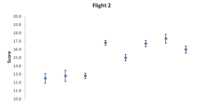
Scores in chart format with dots representing the average score and the bars depicting the spread as a standard error. Wines A through H (left to right).
Statistical sip #4 – Testing the spread
Together, the judges’ individual scores are like repeated measurements of a wine’s quality. The spread of their scores indicates how varied they are. If we were to repeat this tasting another day we may find differences in the scores and spread. But until you gather the time and money to have another tasting, you can use statistics. This way you can determine if the averages you gathered are significantly different from one another so as to determine the winners. One such method is formally known as the ‘Student’s t-distribution’, designed by William Sealy Gosset who coincidently had been applying his statistics knowledge while working at Guinness. Without getting into too much detail, in order to use his method, one needs two objects to compare and a series of repeated measurements of each…The wine scores! Eureka!
The numerical result of this method is called the t-test statistic and it can be converted into a measure called a probability value (p-value) to tell us how much we can be sure the difference between the wine scores in a matchup is not due to mere chance. It represents the level of certainty that we can base our judgement call to determine which one wine scored higher than the other. The smaller the number, the more confident we can be. For example, a p-value of 0.05 tells us that there is a likelihood of ‘5 out of 100’ or ‘1-in-20’ that the difference in score is due to random chance, rather than one wine truly winning out. Most of the time, a 1-in-20 chance is chosen as an arbitrary cut-off. How did the wines fare?
Table 5: Flight 1 – Testing the difference in scores for significance (out of 6 tasters)
| A | B | C | D | E | F | |
|---|---|---|---|---|---|---|
| La Follette | Veramonte | Santa Carolina | Rodney Strong | Gloria Ferrer | Errazuriz | |
| CAL | CHL | CHL | CAL | CAL | CHL | |
| Chard | Chard | Cabsauv | Cabsauv | Pnoir | Pnoir | |
| 17.2 | 11.0 | 13.0 | 16.7 | 16.7 | 14.5 | AVG SCORE |
| 0.6 | 0.4 | 0.5 | 0.6 | 0.3 | 0.2 | SEM |
| Winner CAL p<0.01 | Winner CAL p<0.01 | Winner CAL p<0.01 | t-test p-value (*unpaired and unequal variance) |
Table 6: Flight 2 – Testing the difference in scores for significance (out of 10 tasters)
| A | B | C | D | E | F | G | H | |
|---|---|---|---|---|---|---|---|---|
| Errazuriz Mx | Ch. St. Jean | Cakebread | Maycas Limarí | Chilcas | Dierberg | Dom. Napa | V. San Esteban | |
| CHL | CAL | CAL | CHL | CHL | CAL | CAL | CHL | |
| Svblanc | Svblanc | Chard | Chard | Pnoir | Pnoir | Cabsauv | Cabsauv | |
| 12.5 | 12.8 | 12.8 | 16.8 | 15.0 | 16.7 | 17.3 | 16.0 | AVG SCORE |
| 0.6 | 0.7 | 0.3 | 0.3 | 0.4 | 0.4 | 0.6 | 0.4 | SEM |
| p=0.74 (tie) | Winner CHL p<0.01 | Winner CAL p<0.01 | p=0.09 (tie) | t-test p-value (*unpaired and unequal variance) |
* The term unpaired means that the scores are not partners of each other. In each matchup, we are tasting two separate wines. We might consider a paired test if we tasted the same wine before and after decanting, for example. The test also did not assume that the scores were necessarily going to have an equal spread (unequal variance).
Briefly, in Flight 1, all the scores were in favour of California, but in Flight 2 they were more varied – the Chardonnay clearly went to Chile and the Pinot noir to California. However, the judges were impartial to the Sauvignon and the Cabernet in this flight. So even though the numbers favoured California at face value the differences in the judges’ scores were just not significant enough. It could be that if we had more people to taste the wine maybe we’d have a clearer favourite.
So the last drop of this simple statistics exercise was that the numbers may not always be what they seem. The scores we see with reviews aren’t really meant to take into account the comparative angle. This blind comparison tasting adds a new element to not only our palate but may also add some perspective on how to inform our purchasing choices. From a sensory perspective, in using these scores we can determine whether or not paying a few or many dollars more for a wine is justified. We may even find some value gems.
PART III – You be the judge
And now the fun part –tasting and tallying! Let’s first discuss how the tasting was conducted.
- Separate groups were assembled on two different evenings with eight and 12 participants, respectively.
- Each group had a distinct flight of wines with six in the first group and eight in the second.
- The participants were told only the following facts, with all else being blind.
o The wines are to be tasted in pairs (A vs B, C vs D, and so on), are of the same grape varietal, but one is from California and the other from Chile.
o The wines’ origins are assembled in the flight in random order, so one cannot assume that the first wine of each pair will always be of the same country.
- The participants were then given their score sheets (as in PART 2 of this series) and were asked to grade the wines as well as take an educated guess on the country of origin, grape varietal and estimated retail price as based on their scoring.
- In general, most participants tasted through the flight in alphabetical order and I placed whites ahead of the reds. I suppose I could have randomly arranged all the wines no matter the colour or weight but I did not want the tasters to suffer palate exhaustion so early.
- Some assumptions were that
o Each taster had a rough idea of the total cost of the flight, given the budget per person.
o The tasters understood the retail market enough to know that in general Chilean wines are priced lower than their Californian counterparts. Nevertheless, they were instructed to grade the wines based on quality.
THE WINES
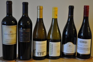
A: 2010 La Follette Lorenzo Vineyard Chardonnay, Russian River Valley, California ($44.95)
B: 2012 Veramonte Reserva Chardonnay, Casablanca Valley, Chile ($12.95)
C: 2010 Santa Carolina Reserva de Familia Cabernet sauvignon, Maipo Valley, Chile ($18.95)
D: 2010 Rodney Strong Reserve Cabernet sauvignon, Alexander Valley, California ($59.95)
E: 2010 Gloria Ferrer Vineyards Pinot noir, Carneros, California ($26.95)
F: 2010 Errazuriz Estate Reserva Pinot noir, Aconcagua, Chile ($13.95)
Flight 2 (8 wines, 12 tasters)
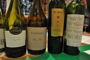
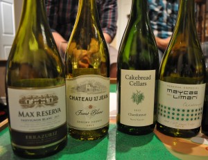
A: 2013 Errazuriz Estate Max Reserva Sauvignon blanc, Aconcagua, Chile ($15.95)
B: 2011 Château St. Jean Fumé blanc (Sauvignon blanc), Sonoma County, California ($19.95)
C: 2012 Cakebread Cellars Chardonnay, Napa Valley, California ($59.95)
D: 2011 Maycas del Limarí Reserva Especial Chardonnay, Limarí Valley, Chile ($19.95)
E: 2011 Chilcas Single vineyard Pinot noir, Maule Valley, Chile ($17.95)
F: 2009 Dierberg Pinot noir, Santa Rita Hills, California ($47.95)
G: 2010 Dominus Estate Napanook Cabernet sauvignon, Napa Valley, California ($77.95)
H: 2011 Viña San Esteban In situ Gran Reserva Cabernet sauvignon, Aconcagua, Chile ($18.95)
So which country won? All is revealed in Part IV.
Search
Recent Posts
- Рабочее Зеркало 1xbet На Сегодня официальному Сайт 1хбет
- Рабочее Зеркало 1xbet На Сегодня официальному Сайт 1хбет
- 1xbet Зеркало Рабочее 1xbet Официальный Сайт вход На Сегодня и 1хбет Казино
- 1xbet Зеркало Рабочее 1xbet Официальный Сайт вход На Сегодня и 1хбет Казино
- 1xbet Вход На официального Сайт Через рабочее Зеркало

